Predicting Freeway Traffic Crash Severity Using XGBoost-Bayesian Network Model with Consideration of Features Interaction

Yang, Yang; Wang, Kun; Yuan, Zhenzhou; Liu, Dan

doi:https://doi.org/10.1155/2022/4257865

Journal of Advanced Transportation

On this page

Abstract Introduction Results and Discussion Conclusions Data Availability Conflicts of Interest Acknowledgments References Copyright Related Articles

Special Issue

Management and Control Methods of Mixed Traffic Flow with Connected Automated Vehicles

View this Special Issue

Research Article | Open Access

Volume 2022 | Article ID 4257865 | https://doi.org/10.1155/2022/4257865

Predicting Freeway Traffic Crash Severity Using XGBoost-Bayesian Network Model with Consideration of Features Interaction

Yang Yang,^1,2Kun Wang,³Zhenzhou Yuan,⁴and Dan Liu⁵

Academic Editor: Gen Li

Received12 Mar 2022

Accepted11 Apr 2022

Published30 Apr 2022

Abstract

In the field of freeway traffic safety research, there is an increasing focus in studies on how to reduce the frequency and severity of traffic crashes. Although many studies divide factors into “human-vehicle-road-environment” and other dimensions to construct models whichshowthe characteristic patterns of each factor's influence on crash severity, there is still a lack of research on the interaction effect of road and environment characteristics on the severity of a freeway traffic crash. This research aims to explore the influence of road and environmental factors on the severity of a freeway traffic crash and establish a prediction model towards freeway traffic crash severity. Firstly, the obtained historical traffic crash data variables were screened, and 11 influencing factors were summarized from the perspective of road and environment, and the related variables were discretized. Furthermore, the XGBoost (eXtreme Gradient Boosting) model was established, and the SHAP (SHapley Additive exPlanation) value was introduced to interpret the XGBoost model; the importance ranking of the influence degree of each feature towards the target variables and the visualization of the global influence of each feature towards the target variables were both obtained. Then, the Bayesian network-based freeway traffic crash severity prediction model was constructed via the selected variables and their values, and the learning and prediction accuracy of the model were verified. Finally, based on the data of the case study, the prediction model was applied to predict the crash severity considering the interaction effect of various factors in road and environment dimensions. The results show that the characteristic variables of road side protection facility type (RSP), road section type (LAN), central isolation facility (CIF), lighting condition (LIG), and crash occurrence time (TIM) have significant effects on the traffic crash prediction model; the prediction performance of the model considering the interaction of road and environment is better than that of the model considering the influence of single condition; the prediction accuracy of XGBoost-Bayesian Network Model proposed in this research can reach 89.05%. The identification and prediction of traffic crash risk is a prerequisite for safety improvement, and the model proposed and results obtained in this research can provide a theoretical basis for related departments in freeway safety management.

1. Introduction

With the continuous improvement of motorization degree, freeway travel demand is increasing, and the freeway has become an important part of the world’s highway transportation system. Due to the driving characteristics of the freeway, once a traffic crash occurs to the vehicle operating on a freeway, it usually has a consequence with a serious casualty or property loss [1]; reducing the severity of traffic crashes is of great significance to improve the safety of the freeway operating. Simultaneously, the occurrence of traffic crashes is sudden and accidental, which is quite difficult to control. Based on this background, exploring the crash precursors of freeway and predicting the severity of freeway traffic crashes has become a popular topic in this field.

Regarding the severity of a roadway traffic crash: studies on influencing factors of crash severity have always been carried out from four dimensions of “human-vehicle-road-environment,” among which the studies on environmental factors, weather and road, account for a large proportion. In order to better understand the influence of weather on traffic crash severity, Satoshi et al. [2] developed a traffic crash severity assessment model based on the ordered Probit model, which took into account traffic characteristics, road conditions, environment, and factors related to multiple vehicles, single vehicles, and bicycles. Lee et al. [3] applied the structural equation model to analyze the relationship between weather conditions and the severity of traffic crashes, and the results showed that the severity of crashes was correlated with the factors of road, traffic, environment, human, rain and water depth on the road, and other factors. Amin et al. [4] studied the impact of climate change on dangerous road crashes related to weather and analyzed the spatiotemporal relationship between weather-related explanatory variables and crash severity index by using negative binomial regression and Poisson regression models; the results showed that the surface weather conditions and weather had a strong positive correlation with the crash severity index, while the road surface form characteristics had a negative correlation with the crash severity index. For the real-time freeway traffic crash analysis, Sun et al. [5] proposed a method of crash risk assessment based on traffic safety state division and quantitatively analyzed the influence of different traffic conditions on freeway crash risk. However, traffic conditions alone may be found to constitute an elevated crash risk, and without an additional behavioral factor to help differentiate the relative risk, the predicted crash risk shall remain low, giving rise to a high proportion of false positive predictions [6]. These above studies analyzed the relationship between subjective or objective factors and the severity of the traffic crash, explained the correlation of the influencing factors by building models, and analyzed whether the influencing factors of each dimension were significantly related to the severity of a crash.

Regarding roadway traffic crash severity prediction research: predicting the severity of road traffic crashes is an important part in the study of roadway traffic safety. The model with high prediction accuracy and accurate prediction results can provide insight for relevant departments to effectively reduce the severity of traffic crashes. In addition to considering different influencing factors, scholars’ research interests mainly focus on using various prediction models to figure out the severity of road traffic crashes, including regression prediction model, Decision Tree, Neural Network, and Bayesian network prediction, etc. [7–10]. Celika et al. [11] analyzed the severity of traffic crashes based on multiple Logit models; in this study, the severity of traffic crashes was divided into fatal accident, injury accident, and noninjury accident, where the results showed that the factors of driver’s education level, road grade, whether there is a crosswalk, crash time, and weather all had a certain impact on the severity of traffic crashes. Jiang et al. [12] adopted the zero-expansion ordered Probit model to study the influence of traditional influencing factors such as kerb and speed limit changes on the severity of single-vehicle collision crash. Shaheed et al. [13] applied the mixed Logit model to the construction of the crash severity prediction model and analyzed whether various factors had a significant influence on the crash severity. The study was based on motorcycle crash data in Iowa State, USA; the crash severity was classified into five categories: fatal, major injury, minor injury, possible or unknown, and PDO (property damage only). Lou [14] analyzed the risk states of freeway under different time conditions and proposed a traffic crash severity prediction method based on the mixed Logit model. Alkheder et al. [15] used three data mining models, including decision tree, linear support vector machine, and Bayesian network model, to analyze the risk factors related to traffic crash severity, and the performance of the application model showed that Bayesian network predicted variables more accurately than other models. In general, the study of Bayesian network has been introduced into the field of traffic crash severity prediction, and compared with regression models, decision tree, and other models, Bayesian network prediction is typically more accurate.

Based on the above analysis, there are many existing studies which analyzed the influence of weather or road on crash severity or comprehensively analyzed the influence of road and environmental factors, but there is a lack of research considering the influence mechanism of interaction between road dimension factors and environmental dimension factors on traffic crash severity prediction. In order to achieve a more accurate prediction for the severity of freeway traffic crashes, identify the main risk factors of freeway traffic crashes, and reduce the freeway crash severity, this research takes freeway operation as the research object. In this research, XGBoost model is constructed and SHAP value is introduced to interpret the model results. The global impact and importance ranking of each characteristic factor on the severity of the crash are obtained through the interpretation results of SHAP values, and the impact degree of a single variable on the severity of the crash and the interaction effect between independent variables are obtained. The prediction model of freeway traffic crash severity is determined by the inference model based on clip-tree propagation algorithm; finally, the traffic crash severity is predicted considering the interaction effect between road and environment.

2. Data Process

2.1. Data Source

In this research, traffic crashes on freeways in Hebei Province, China, in 2018 are taken as the research object. The dataset used in this research includes a total of 567 pieces of crash data, covering 35 attribute variables. Table 1 describes the summary of attribute variables in the raw dataset.

2.2. Data Variables Selection

Most of the studies involving the severity prediction of freeway traffic crashes basically include the selection of influencing factors from four aspects: human-vehicle-road-environment. However, some studies only selected some of the factors from some dimensions to predict and analyze the crash severity. For example, Ma et al. [16] selected 12 candidate objective independent variables from the aspects of time, road, and traffic operation environment in order to avoid excessive attention to human factors while ignoring the impact of objective factors on traffic crashes and established a cumulative logistic model to analyze their impact on the severity of traffic crashes. Through the goodness of fit and prediction accuracy test of the model, the model fitting effect performed better, and the modeling conclusion had a certain practical reference significance. Hence, the establishment of a prediction model based on the influence of objective factors also has a certain research significance. Consequently, based on the sample dataset, this research screens out the influencing factors of road and environment, mainly exploring the influence of road and environment factors on crash severity. Table 2 gives the influencing variables of freeway traffic crash severity in this research. Since the selected factor variables include attribute variables and continuous variables, they need to be discretized to meet the requirements of modeling.

3. Screening Influence Factors Based on XGBoost

3.1. The Fundamentals of XGBoost

Boosting library XGBoost [17, 18] is a boosting library developed by Chen in 2016, which is an improvement of the gradient lifting algorithm. Gradient lifting algorithm does not only have a gradient lifting tree; thus, the weak estimators in XGBoost algorithm can also choose linear models such as logistic regression and linear regression in addition to the tree model. However, XGBoost technically uses the tree model for integration. In many machine learning algorithms, the loss function is used to measure the generalization ability of the model, that is, the prediction accuracy of the model on unknown data, and the calculation speed of the model cannot be measured. XGBoost algorithm achieves a balance between model performance and model operation speed; it combines the prediction accuracy of the model with engineering capability. In addition to the loss function, model complexity is also introduced into the objective function of XGBoost algorithm to measure the operation efficiency of the algorithm [19, 20]. Its objective function is as follows:

For the freeway traffic crash data set, where i represents the i-th crash sample in the dataset, the first item represents the loss function of the model, which measures the difference between the real value y_i and the predicted value of the crash severity. The loss function can be selected according to the predicted demand. The second term is the regularization term, which represents the complexity of the model. It is represented by some transformation Ω of the tree model, which means that the complexity of the tree model is measured from the structure of the tree. The approximate target is obtained by Taylor expansion [19, 20], which is

Define expression:

The second-order Taylor expansion of the loss function can be obtained as

The second partial derivative Taylor expansion in XGBoost has a strong advantage, which makes the gradient descent faster and more accurate. The second derivative form of the function as an independent variable is obtained according to Taylor expansion; the specific form of the loss function does not have to be selected, but it only depends on the value of the input data for calculation, which increases the compatibility of the model.

3.2. Model Interpretation Based on SHAP

Compared with conventional linear models, XGBoost has improved the prediction accuracy. However, it loses the interpretability that linear models have; thus, it is almost considered as a black box model. Lundberg et al. [21] proposed the method of SHAP value in order to interpret various models (classification and regression) including the black box model.

SHAP is an additive interpretation model inspired by Shapley values. In the prediction model, each prediction sample will generate the corresponding prediction value, and the value assigned to each feature in the sample is SHAP value. Assume that the ith sample is x_i, the jth feature of the ith sample is x_ij, the predicted value of the model for the ith sample is y_i, and the baseline of the whole model is (basically it is the mean of the target variable of all samples); hence the SHAP value follows the following formula [22]:where f (x_i, 1) denotes the SHAP value of the first feature of the ith sample, that is, the contribution value of f (x_i, 1) to the predicted value y_i. When f (x_i, 1) > 0, it means that this feature improves the predicted results; that is, it has a positive effect; otherwise, it has a negative effect, which means that this feature reduces the predicted value.

“Feature importance” was previously used to explain the XGBoost model. This method is applied to measure the importance of each feature in the dataset to the model and determine which features have a greater impact on the final model, but the relationship between features and predicted results cannot be determined. Not only can SHAP values reflect the influence degree of each feature in each sample on the model, but it is able to show the positiveness and negativity of the influence, which is the advantage of using SHAP value to interpret the model [22].

3.3. XGBoost Hyperparameter Optimization

In this research, Grid Search CV is introduced to search the optimal parameter value of the model, among which, “Learning_rate” (update shrinkage step in the learning process), “max_depth” (maximum depth of tree), “n_estimators” (control number of weak estimators), and “subsample” (random sampling ratio), which have great influence on the model performance, are selected for optimization searching, where “learning_rate” typically ranges from 0.0 to 0.05 and the “search step” is 0.01. “Max_depth” typically ranges from 3 to 11 and the “search step” is 1. “N_estimators” typically ranges from 100 to 400 and the “search step” is 50. The candidate values of “subsample” are 0.7, 0.8, and 0.9.

Firstly, the data is imported, and the regression prediction model is established, and any candidate values are selected as the initial values of parameters. After the model is established, the parameter optimal solution of the model is searched by using the hyperparameter meshing optimization function, and the model optimization result is learning_rate = 0.04, max_depth = 3, n_estimators = 100, subsample = 0.9. The optimal parameters are reinput into the model to obtain the optimal solution model, and then the SHAP interpreter is built. The interpretation of SHAP on the model results is visualized, and the global influence and importance ranking diagram of each factor variable on the severity of the traffic crash can be output.

3.4. XGBoost Hyperparameter Optimization and Model Interpretation Analysis

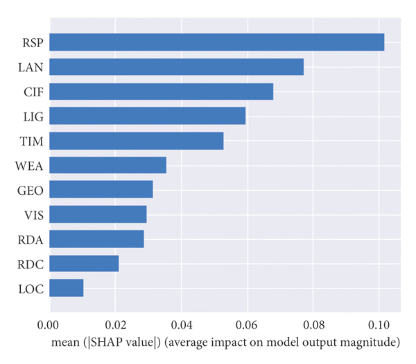
First, the data is imported, and the regression prediction model is established. Then, any candidate value is selected as the initial parameter value. After the model is established, the optimal parameter solution of the model is searched by using the hyperparametric gridding optimization function. The optimization results of the model are learning_rate = 0.04, max_depth = 3, n_estimators = 100, subsample = 0.9. Reinput the optimal parameters into the model to obtain the optimal solution model, and then build the SHAP interpreter to visualize the interpretation of SHAP to the model results. The global impact and importance ranking of each factor variable on the traffic crash severity can be output as shown in Figure 1.

(a)

(b)

Figure 1(a) shows the contribution degree of feature factors to the severity degree of the traffic crash. Here, the importance of features is sorted according to the mean value of the absolute value of the impact degree of feature on the target variable. It can be seen from the figure that the variable RSP has the greatest global impact on the severity of the crash; that is, it has the greatest contribution to the prediction result of the freeway traffic crash severity. Additionally, LAN, CIF, LIG, and TIM also have great impact on the prediction.

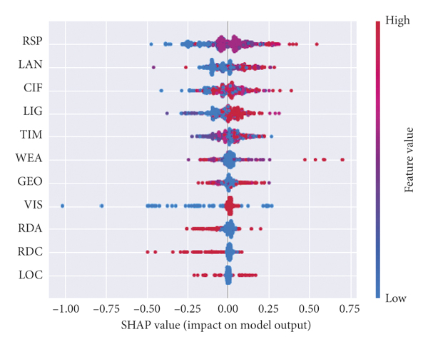
Figure 1(b) shows the tendency of influencing factors to different traffic crash severity. Each row in the figure denotes a feature factor, the horizontal coordinate represents the SHAP value, each dot represents a sample, and the color of each dot denotes the value of the corresponding feature. From blue to red, the value of the feature itself is getting bigger. Smooth color transitions of SHAP values can be observed horizontally as changes in the values of the feature itself and the influence of the feature gradually alter the output of the model.

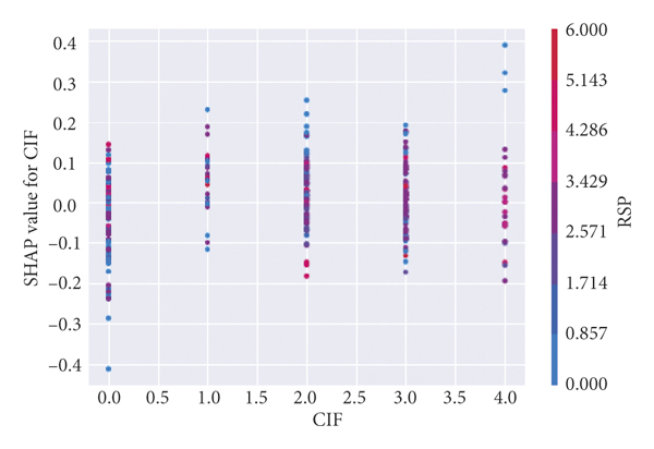
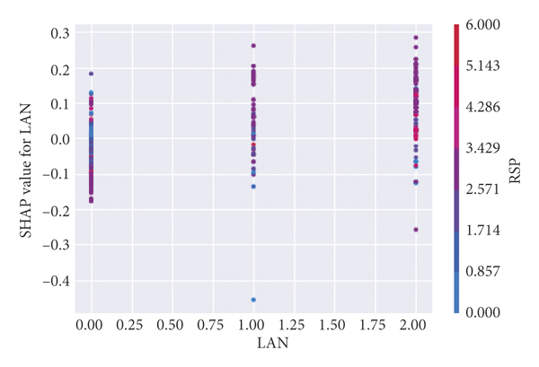
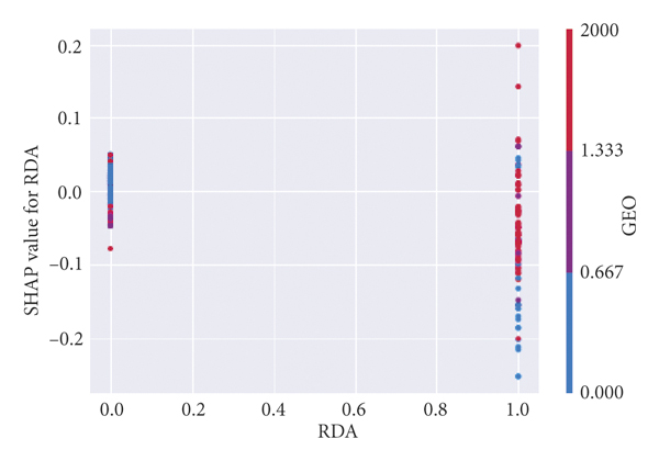
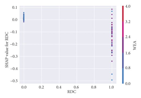
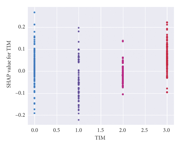
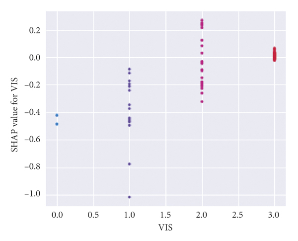
Figure 2 specifically reflects the influence of each characteristic independent variable value on the traffic crash severity of the dependent variable. The abscissa is the value of the independent variable, and the ordinate is the SHAP value, which is the contribution value of the feature to the prediction result of the crash severity. There are deputy ordinates in Figures 2(a)–2(d), which indicates that there are collinearity problems between CIF and RSP, LAN and RSP, RDA and GEO, ROC and WEA. The figure reflects the interaction effect between the two collinear independent variables and their contribution degree to the prediction results of crash severity, indicating that the model used in this research can deal with the collinearity problem well, and the collinear independent variables will not affect the fitting of the model. For example, as shown in Figure 2(a), the SHAP value of CIF does not change significantly under various CIF values, and the VALUE of CIF is large. That is, when the central isolation is metal guardrails and green belts, roadside protection facilities are generally metal guardrails, green belts, and roadside trees.

(a)

(b)

(c)

(d)

(e)

(f)

(g)

(h)

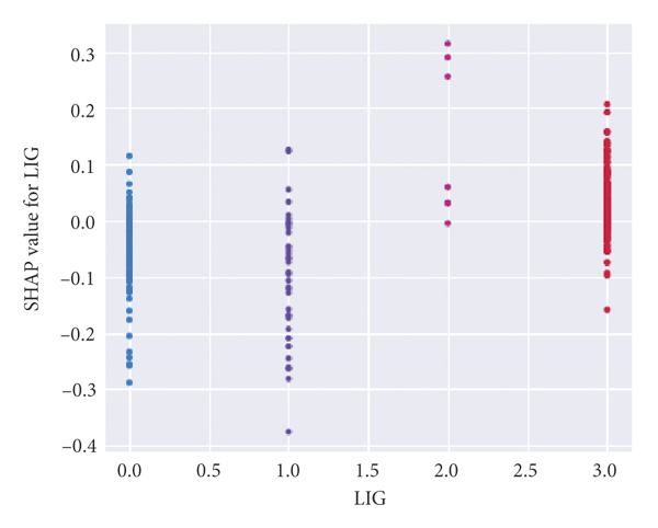
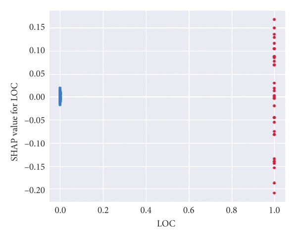
Figures 2(e)–2(h) reflect the relationship between a single variable and the severity of the traffic crash.

Figure 2(e) illustrates that when the lighting condition is daytime, dusk, or dawn, SHAP value is basically less than 0, which may reduce the value of crash severity; that is, slight severity crashes are more likely to occur. When the lighting condition is night with lighting or night without lighting, SHAP value is basically greater than 0, which has a positive promoting effect towards the occurrence of serious crashes.

Figure 2(f) illustrates that the proportion of crashes that occurred in the carriageway is large; concurrently, the severity of crashes is evenly distributed in both carriageway and noncarriageway.

Figure 2(g) shows that when the value of TIM is 3, that is, during 18:00∼24:00, the corresponding SHAP value is basically concentrated on the side greater than 0, which has a positive promoting effect on the occurrence of serious crashes.

Figure 2(h) indicates that most of the crashes occurred when the visibility value is 3; that is, when the visibility is above 200 meters, SHAP value greater than 0 has a positive effect on serious crashes.

Figure 3 illustrates the interaction of multiple variables. There is an interaction effect between RSP and LAN. However, the interaction effect is not a simple linear relationship. When the red dots are mainly concentrated on the side with SHAP values less than 0 and the blue dots are mainly concentrated on the side with SHAP values greater than 0, RSP is negatively correlated with LAN. There is a certain threshold, and when the interaction between RSP and LAN exceeds this threshold, the correlation gradually shows positive. LAN and CIF have an interaction effect and weak positive correlation. The nonlinear interaction between LIG and RSP, and LIG and WEA also exists. There are interaction effects between GEO and CIF and a weak positive correlation between GEO and RDA. There are interaction effects between GEO and RDC and a weak negative correlation between LAN and RDC. RDA and LAN, and RDA and TIM have interactive effects and positive correlations. There is almost no interaction between the other two variables, and their sample distribution is random.

4. Modeling of Bayesian Network

Bayesian network has a strong probability theory foundation and strong explanatory ability through graph theory; hence some uncertain problems in many fields can be solved via Bayesian methods, such as fault diagnosis, pattern recognition, and accident prediction, etc. [23]. The content of this research is traffic crash severity prediction; since the occurrence of traffic crashes is uncertain, the content also belongs to the uncertain inference problem [24]; using Bayesian network is effective to the advantage of uncertainty inference and can build a relatively accurate inference model and realize effective prediction of the severity of traffic crashes.

4.1. Validation of Bayesian Network Learning Results

The data sample information used in this study is complete, and there are many node variables selected; therefore, the structure learning method based on scoring search is picked. The structure learning method based on score search includes two parts: one is to select an appropriate score function to evaluate the quality of the network structure; the other is to determine the appropriate search strategy for finding the highest rated network structure. The scoring function selected in this research is the BD scoring function based on Bayesian statistics, which has good accuracy and fitting effect. K2 search algorithm is a commonly used search strategy for searching high-scoring network structures, which combines the selected scoring function and search strategy to search for the optimal network structure [25].

K2 search algorithm uses greedy search to obtain the maximum score function. When the K2 search algorithm is applied to learn the structure search of Bayesian network, it is necessary to determine the node order in advance. Given the order, the search range can be reduced, and the maximum number of parent nodes in the network should be given first, which is a constraint on the search optimization and can improve the search efficiency. After determining the order of nodes, consider any node in the network; if the node X_i is before node X_j, the network edge cannot exist from Xj to X_i. According to the order of network nodes and the maximum number of parent nodes, the node with the maximum value of the scoring function is selected as its parent node. When the scoring function can no longer increase, the loop is stopped. The specific optimization algorithm flow is shown in Algorithm 1.

	Input: node variable set “n,” node order “order,” maximum number of parent nodes “Max_fan_in,” observation data set “D.”
	Output: Optimal network structure based on K2 algorithm, that is, each point and its parent node.
(1)	for i = 1 to n (n represents the number of total nodes);
(2)	π _i = ∅;
(3)	p _old = (i, π_i);
(4)	Set variable OKTOProceed = true;
(5)	while OKTOProceed = true and \|π_i\| < m do;
(6)	pick one node z from p_red (i) − π_i, let (i, π_i {z}) maximize, where p_red (i) denotes the nodes whose order is before the ith node;
(7)	Calculate ;
(8)	If then;
(9)	;
(10)	;
(11)	;
(12)	else ;
(13)	end while;
(14)	return (node , parent node );
(15)	end for;
(16)	end K2.

Since the order of network nodes is required to be given when the K2 search algorithm is used for structure learning to reduce the search range, the determination of the order of network nodes is mostly based on the correlation analysis results of independent variables and dependent variables in previous studies [26]. The determination of node order is a subjective decision process, and the variables have an interaction effect with each other. It is not proper to determine the node order via analyzing the correlation between independent variables and dependent variables; the input of such network node order will affect the result of Bayesian network structure learning. Therefore, it is necessary to address this problem by the proposed approach in this research considering the interaction effect of features.

In this research, the order of network nodes is determined based on the interpretation results of XGBoost model by SHAP. XGBoost model is used to analyze the factors influencing the severity of freeway traffic crashes, and SHAP is used to explain the model to obtain the order of the importance of the global impact of each characteristic variable on the crash severity. The importance degree from large to small is type of road side protection facilities, type of road section, central isolation facilities, lighting conditions, accident time, weather, terrain, visibility, road alignment, road surface, and road section location.

Figure 4 depicts a thermal diagram of correlation coefficients between variables. According to the correlation coefficient between each independent variable and the decision variable in the figure, all variables are sorted in order from large to small: roadside protective facilities type, road type, lighting conditions, geography, road alignment, road surface conditions, weather, visibility, accident time, central isolation facilities, and road section location.

In the order obtained from the correlation of sorting, the impact of road surface conditions on the severity of crashes contributes more than that of weather; this is indeed unreasonable, because road surface conditions are largely influenced by the weather. Based on the preceding content about the interaction between the variables’ effect diagram, we can see the weather and road conditions have a significant positive correlation. Therefore, the influence of weather on the severity of the crash is greater than that of the road surface condition. It can be seen that the importance ranking obtained by the proposed approach in this research is relatively reasonable.

According to the above analysis, the order of node variables is determined as follows: 1- road section location, 2- road surface condition, 3- road alignment, 4- visibility, 5- geography, 6- weather, 7- accident occurrence time, 8- lighting conditions, 9- central isolation facilities, 10- road section type, 11- road side protection facilities type, 12- crash severity. For the obtained Bayesian network, the validity analysis is needed to ensure that the Bayesian network inference model is accurate. Then the validity of the constructed network is verified from the aspect of learning accuracy of Bayesian network. The error of parameter learning can be obtained by comparing the statistical calculation results in the sample with the node parameter learning results in the Bayesian network. The learning accuracy of the Bayesian network can be inferred from the parameter learning error [27]. The decision variable in this research is the traffic crash severity; thus, the parameter learning results of the node of crash severity are used to verify. The learning results of node parameters of decision variables are compared with the statistical results of sample data; the absolute error and relative error between them are calculated to judge the learning effect. Due to the large number of types of roadside protection facilities directly affecting decision variables [28], the comparison results cannot be fully displayed. Therefore, the comparison results of fatal crashes are selected for analysis. Specific calculation results are shown in Table 3.

The maximum absolute error of parameter learning results is less than 6%, while the maximum relative error is mostly within 5%. Although the learning accuracy of the model network structure is not very high, the network model still has certain reference significance. The reason affecting the training accuracy probably is that the sample size of crash data is small.

4.2. Construction and Verification of Bayesian Network Inference Model

After the Bayesian network structure is obtained, the inference operation engine in the full-BNT toolbox of MATLAB software is called on the basis of this structure to obtain the Bayesian network inference model. The expected probability distribution of the desired nodes can be figured out by inputting the values of any one or more network nodes in the inference model. The node to be speculated in this research is the severity of the traffic crash, so the query variable in the model can be set to the traffic crash severity. When the values of other node variables or combinations of variables are known, the probability distribution of traffic crash severity can be calculated according to the model; that is, the severity of the crash can be predicted. The inference method selected in this research is the more commonly used and efficient clip-tree propagation algorithm, which belongs to precise reasoning, and the corresponding operation engine in the toolbox is “Jtree_INF_engine.” Figure 5 shows the inference process.

4.2.1. Constructing the Moral Graph

Constructing the moral graph is the first step of Bayesian network inference based on clip-tree propagation algorithm. In this process, the direction of each directed edge in the directed acyclic graph is removed, and then each parent node in the network is combined. The undirected graph is the moral graph. After getting the initial moral graph, check whether each node is in the triangle region. If the most simplified region of the node is the polygon region, then remove the polygon by adding edges. Finally, make each node in the triangle region, and get the final moral graph of the network. Figure 6 is the moral graph of the constructed Bayesian network for freeway traffic crash severity.

4.2.2. Determining the Elimination Order of Variables

According to the moral graph, the maximum potential search method can be adopted to determine the order of variables elimination. The working principle of the maximum potential search method is that, on the basis of determining the eliminated variables, the selection of the next variable can minimize the correlation potential between variables. The specific process is as follows: firstly, select any node and mark it, then find the unmarked node that is connected to the most marked nodes, and continue marking. If there are multiple nodes with the most adjacent marked nodes, select any node to continue marking. When all nodes are marked, the nodes are sorted according to the marked order, with the first marked in the last and the last marked in the first. The resulting node order is the optimal elimination order of variables. Generally, any root node in the Bayesian network is selected as the starting marker, and the elimination order of variables according to the above search method is 12 ⟶ 9 ⟶ 2 ⟶ 3 ⟶ 10 ⟶ 7 ⟶ 5 ⟶ 4 ⟶ 6 ⟶ 8 ⟶ 11 ⟶ 1.

4.2.3. Constructing the Cluster-Tree

After determining the elimination order of variables, the elimination of variables is carried out according to the elimination order starting from the Bayesian network moral graph. Before eliminating the nodes, a clique consisting of the variable to be eliminated and all variables adjacent to that variable is constructed until all variables are eliminated in order. After elimination, the resulting cliques are organized in an appropriate way to obtain a cluster-tree containing all nodes. Via this approach, a Bayesian network cluster-tree of freeway crash severity is constructed, and the results are shown in Figure 7.

4.2.4. Setting Inferential Evidence

Given the information of any node variable, the tree can effectively transfer and share the information of the node after constructing the cluster-tree according to the above way. The efficiency of cluster-tree propagation algorithm lies in its real-time information sharing, which can simplify the transfer process between cluster-tree and inference process. Before inferential analysis, the evidence variables should be given first, and then the query variables should be determined. The evidence variable and query variable can be one or a combination of multiple variables. The query process of multiple query variables uses the shared inference mechanism of cluster-tree to deduce the results of multiple query variables, based on the inference of query variables. After determining the query variable and the evidence variable, the correlation between the evidence variable and the query variable can be figured out according to the conditional probability and Bayesian theorem.

The sequence of nodes of Bayesian network of freeway traffic crash severity established in this research is as follows: [TIM] [LOC] [RDC] [RDA] [LAN] [CIF] [RSP] [GEO] [WEA] [VIS] [SEV]. The purpose of constructing Bayesian network inference model is to deduce the severity of traffic crash. Therefore, “SEV” is set as the query variable in this research, which belongs to single-query variable inference. The selection of evidence variables can be any combination of the first 11 node variables.

4.2.5. Inference Learning

The inference solution process of Bayesian network is based on conditional probability and Bayesian theorem. In this research, the prediction model of crash severity is constructed via the toolbox “FULL-BNT” in MATLAB software, which integrates the learning and inferring algorithm functions of Bayesian network. The specific inference process is as follows: Input the previously obtained Bayesian network, then use the joint tree inference engine “jtree _ inf _ engine (bnet)” in FULL-BNT toolbox to build the inference model, and finally input evidence variables and query variables to carry out inference learning. What this research expects to predict is the traffic crash severity; thus the query variable is set as SEV. After obtaining the inference model based on the above work, the probability distribution of crash severity can be figured out by the inference prediction model by inputting the values of other expected node variables into the inference program.

4.2.6. Validation of the Model Accuracy

The specific process of calculating the prediction accuracy of the model in MATLAB is as follows: First, import the existing sample data and input values of the other 11 dependent variables corresponding to each crash data into the prediction model, that is, input evidence variables; then, the predicted results of crash severity are compared with the actual severity of the corresponding crash data, and the severity of all sample data is predicted in turn; the ratio analysis is processed towards the correctly predicted quantity of traffic crashes with the quantity of all crashes; finally, the accuracy of the prediction model is carried out.

The realization for this part of the work needs to design verification programs in MATLAB and then go through 557 pieces of crash data, in which 496 crashes are accurately predicted; hence the prediction accuracy of the model is 89.05%. When the prediction accuracy of the model is greater than or equal to 80%, the prediction results of the model are relatively good [19]. Therefore, it can be seen that the traffic crash severity prediction model constructed in this research has good prediction accuracy.

5. Results and Discussion

Considering the influence of the interaction of various factors on the severity of crashes, the influence rule of these factors on the traffic crash severity is obtained by analyzing the inference results of the prediction model, which can provide a direction for the follow-up traffic safety management countermeasures.

5.1. Interaction between Weather and Road Type

Input values of weather and road type in the prediction model. Set the variables as Evidence {WEA} = I, Evidence {LAN} = j, where I ranges from 1 to 5 and j ranges from 1 to 3. The output results of the model are the prediction results of accident severity under the corresponding weather variables and road section type variables, and the specific contents are shown in Table 4.

Road section types have a certain influence on the three types of traffic crashes, among which the influence on property loss crashes is relatively greater. When the road type is a complex node (ramp, road entrance and exit, etc.), the probability of injury crash is lower than other road types under any weather condition; synchronously, the probability of property loss and fatal crash is relatively increased. This is consistent with the inference result of single factor analysis [19].

By analyzing the inference results of the two variables on injury crashes, it can be seen that injury crashes are most likely to occur in foggy conditions of special road sections. By analyzing the inference results of property loss crashes, it can be seen that the possibility of property loss crashes in complex node sections is greater than other sections under any weather conditions; in particular it is the greatest in foggy conditions. It can be seen from the analysis of the inference results of two variables on fatal crashes that the probability of fatal crashes is the highest in rainy days at ordinary road sections, while the analysis results towards single factor influence in the previous section of this paper show that the probability of fatal is the highest in complex node crashes and the probability of fatal crashes is the highest in rainy days.

5.2. Interaction between Weather and Road Alignment

Input evidence values of weather and road alignment; the settings are as follows: evidence {WEA} = i, evidence {RDA} = j, where i ranges from 1 to 5 and j ranges from 1 to 2. The output results of the model are the prediction results of crash severity under the corresponding weather variables and road alignment variables, and the specific contents are shown in Table 5.

The results in Table 5 indicate that the interaction of the two variables has an impact on all three types of crashes, among which the impact on injury and death is relatively greater. For the road alignment, the possibility of injury crash occurring in nonstraight alignment is greater than that in straight alignment, while the possibility of a fatal crash occurring in nonstraight alignment is greater than that in straight alignment, which is consistent with the law of road alignment affecting the severity of crashes by a single factor [19].

By analyzing the inference results of the two variables to the property loss crash, it can be seen that the property loss crash is most likely to occur in the foggy days of nonstraight road section. By analyzing the inference results of the two variables on injury crashes, it can be seen that injury crashes are most likely to occur in foggy conditions of nonstraight sections. It can be seen from the analysis of the inference results of fatal crashes that the possibility of fatal crashes is the greatest in the case of straight sections under snowy conditions, and the possibility of fatal crashes is relatively greater in the case of straight sections under rainy conditions, which is basically consistent with the influence rule of the single factor on the crash severity [19]. Therefore, the interaction effect of weather and road alignment on the severity of crashes is not obvious.

5.3. Interaction between Road Alignment and Crash Time

The evidence variables’ values of road alignment and crash occurrence time are input into the prediction model. The settings are as follows: evidence {RDA} = i, evidence {TIM} = j, where the value of i ranges from 1 to 2 and the value of j ranges from 1 to 4. The output results of the model are the prediction results of crash severity under the corresponding road alignment variables and crash occurrence time variables, and the specific contents are shown in Table 6.

The interaction of road alignment and crash occurrence time on the severity of the accident is analyzed. Combined with the inference results in Table 6, it can be seen that the interaction of the two variables has a certain impact on the severity of the three types of crashes; among them, the impact of property loss crash and fatal crash is relatively greater. By analyzing the inference results of the two variables on property loss crash and injury crash, it can be seen that when the road alignment is not straight and the time is during 12:00 to 18:00, the probability of property loss crash or injury crash is the largest. It can be seen from the analysis of the inference results of the two variables to the fatal crash that when the road alignment is not straight and the occurrence time is 18:00 ∼ 6:00, the probability of fatal crashes accounts the largest on the nonstraight road at night.

5.4. The Interaction between Weather and Lighting Conditions

Enter the values of the evidence variables weather and lighting conditions into the prediction model; set the variables as evidence {WEA} = i, evidence {LIG} = j, where the value of i ranges from 1 to 5 and the value of j ranges from 1 to 4. The output results of the model are the prediction results of crash severity under the corresponding weather variables and lighting condition variables, and the specific contents are shown in Table 7.

The influence rules of weather and lighting conditions on the severity of crashes are analyzed. According to the inference results in Table 7, it can be seen that the interaction of the two variables has a great influence on the severity of the three types of crashes. In terms of lighting condition, the possibility of property loss crash is the greatest (including all weather conditions), and the overall probability of fatal crashes occurring when there is no lighting at night is the highest, while the overall probability of fatal crash occurring when there is lighting at night is the highest, which is basically consistent with the results of single factor analysis [19].

By analyzing the inference results of the two variables on property loss and injury crashes, it can be seen that the possibility of property loss and injury crashes on a foggy night with lighting is greater than that in other weather and lighting conditions. By analyzing the inference result of fatal crashes, the possibility of fatal crash is greater when it is sunny or rainy and there is lighting at night. The univariate analysis results show that the probability of injury crashes is high on foggy days, while the probability of fatal crash is high on rainy days [19]. Therefore, the interaction between weather and lighting conditions has no significant change on the law of traffic crash severity.

6. Conclusions

This research considers the influence of road and environmental factors on the severity of freeway traffic crashes, uses XGBoost to determine the importance of features, and establishes a Bayesian network model to analyze the prediction of traffic crash severity under the interaction of road and environmental factors. The main conclusions are as follows:(1)Inclement weather conditions such as rain, snow, and fog occur in most of the combined conditions of fatal crashes; the nonguardrail form of roadside protection facilities, such as green belt and road trees, is more likely to cause fatal crashes; foggy days have great influence on property loss and injury crashes. Rainy days are the most likely to cause fatal crashes. The interaction between ordinary road sections and rainy days has a great influence on the crash severity. Driving on nonstraight roads at night may aggravate the severity of the crash.(2)In this research, XGBoost-SHAP value model is introduced in the learning of Bayesian network structure to obtain the global importance ranking of each variable on decision variables. Compared with the order of importance obtained from correlation analysis, the determination of the order of variable importance is more reasonable, which is conducive to obtaining a higher scoring Bayesian network structure.(3)Partial results obtained by the traffic crash severity prediction method considering the features interaction effect proposed in this research consist of some of the results obtained by considering only a single factor model in previous studies, indicating that the model used in this research is reliable. Additionally, since the crash-prone variables have an interaction effect with each other, the model with the consideration of features interaction can produce more reliable results. Finally, corresponding effective measures can be put forward to prevent the occurrence of crashes or reduce the crash severity according to the combination form of road and environmental factors with higher risk coefficient, which can be applied by the relative transportation department for the freeway safety management.(4)The amount of sample data used in this research is small, and the factor variables in the dimension of road condition in the used dataset are not complete enough. Furthermore, before learning the structure of the Bayesian network, further research into how to eliminate the influence of small datasets on Bayesian network model construction should be completed and addressed in future models.

Data Availability

Some or all data, models, or codes that support the findings of this study are available from the corresponding author upon reasonable request.

Conflicts of Interest

The authors declare that they have no known competing financial interests or personal relationships that could have appeared to influence the work reported in this paper.

Acknowledgments

This work was supported by China Postdoctoral Science Foundation (2021M700333), Open Project of Shandong Key Laboratory of Highway Technology and Safety Assessment (SH202105), and Beijing Natural Science Foundation (J210001).

References

A. T. Kashani and K. Zandi, “Influence of traffic parameters on the temporal distribution of crashes,” KSCE Journal of Civil Engineering, vol. 24, no. 3, pp. 954–961, 2020.
View at: Publisher Site | Google Scholar
S. Hyodo and K. Hasegawa, “Factors affecting analysis of the severity of accidents in cold and snowy areas using the ordered probit model,” Asian Transport Studies, vol. 7, Article ID 100035, 2021.
View at: Publisher Site | Google Scholar
J. Lee, J. Chae, T. Yoon, and H. Yang, “Traffic accident severity analysis with rain-related factors using structural equation modeling - a case study of Seoul city,” Accident Analysis & Prevention, vol. 112, pp. 1–10, 2018.
View at: Publisher Site | Google Scholar
M. S. R. Amin, A. Zareie, and L. E. Amador-Jiménez, “Climate change modeling and the weather-related road accidents in Canada,” Transportation Research Part D: Transport and Environment, vol. 32, pp. 171–183, 2014.
View at: Publisher Site | Google Scholar
D. Sun, Y. Ai, Y. Sun, and L. Zhao, “A highway crash risk assessment method based on traffic safety state division,” PLoS One, vol. 15, 2020.
View at: Publisher Site | Google Scholar
S. Roshandel, Z. Zheng, and S. Washington, “Impact of real-time traffic characteristics on freeway crash occurrence: systematic review and meta-analysis,” Accident Analysis & Prevention, 2015.
View at: Publisher Site | Google Scholar
Y. Ci, H. Wu, Y. Sun, and L. Wu, “A prediction model with wavelet neural network optimized by the chicken swarm optimization for on-ramps metering of the urban expressway,” Journal of Intelligent Transportation Systems, vol. 26, no. 3, pp. 356–365, 2022.
View at: Publisher Site | Google Scholar
M. A. Rahim and H. M. Hassan, “A deep learning based traffic crash severity prediction framework,” Accident Analysis & Prevention, vol. 154, no. 1, Article ID 106090, 2021.
View at: Publisher Site | Google Scholar
Q. Zeng, H. L. Huang, P. P. Xu, and M. Ma, “Developing an optimized artificial neural network to predict traffic crash injury severity,” in Proceedings of the Cota International Conference of Transportation Professionals, Changsha, China, July 2014.
View at: Publisher Site | Google Scholar
X. Chen, H. Chen, Y. Yang et al., “Traffic flow prediction by an ensemble framework with data denoising and deep learning model,” Physica A: Statistical Mechanics and its Applications, vol. 565, Article ID 125574, 2021.
View at: Publisher Site | Google Scholar
A. K. Çelik and E. Oktay, “A multinomial logit analysis of risk factors influencing road traffic injury severities in the Erzurum and Kars Provinces of Turkey,” Accident Analysis & Prevention, vol. 72, pp. 66–77, 2014.
View at: Publisher Site | Google Scholar
X. Jiang, B. Huang, R. L. Zaretzki, S. Richards, X. Yan, and H. Zhang, “Investigating the influence of curbs on single-vehicle crash injury severity utilizing zero-inflated ordered probit models,” Accident Analysis & Prevention, vol. 57, pp. 55–66, 2013.
View at: Publisher Site | Google Scholar
M. S. B. Shaheed, K. Gkritza, W. Zhang, and Z. Hans, “A mixed logit analysis of two-vehicle crash severities involving a motorcycle,” Accident Analysis & Prevention, vol. 61, pp. 119–128, 2013.
View at: Publisher Site | Google Scholar
C. Lou, Analysis of Causes and Severity of Freeway Traffic Accidents Based on Time and Space, Beijing Jiaotong University, Beijing, China, 2021, In Chinese.
S. AlKheder, F. AlRukaibi, and A. Aiash, “Risk analysis of traffic accidents’ severities: an application of three data mining models,” ISA Transactions, vol. 106, pp. 213–220, 2020.
View at: Publisher Site | Google Scholar
Z. Ma, C. Shao, and C. Dong, “Temporal-spatial analysis model of traffic accident severity based on cumulative logistic model,” China Safety Science Journal, vol. 21, no. 9, pp. 94–99, 2011, In Chinese.
View at: Publisher Site | Google Scholar
T. Chen and C. Guestrin, “XGBoost: A Scalable Tree Boosting System,” in Proceedings of the 22nd ACM SIGKDD International Conference on Knowledge Discovery and Data Mining, San Francisco, CA, USA, August 2016.
View at: Google Scholar
R. Hortegal, Y. Maduro, R. Cancellier et al., “Mechanical dispersion of left ventricle and left atrial reservoir strain are both superior to global longitudinal strain to predict exercise capacity in heart failure with preserved ejection fraction,” European Heart Journal - Cardiovascular Imaging, vol. 23, 2022.
View at: Publisher Site | Google Scholar
C. Li, X. Wu, Z. Zhang, Z. Ma, Y. Zhu, and Y. Chen, “Freeway traffic accident severity prediction based on multi-dimensional and multi-layer Bayesian network,” in Proceedings of the 2022 IEEE 2nd International Conference on Power, Electronics and Computer Applications (ICPECA), pp. 1032–1035, Shenyang, China, January 2022.
View at: Publisher Site | Google Scholar
S. Sun, C. Zhang, and G. Yu, “A Bayesian network approach to traffic flow forecasting,” IEEE Transactions on Intelligent Transportation Systems, vol. 7, no. 1, pp. 124–132, 2006.
View at: Publisher Site | Google Scholar
S. M. Lundberg, G. G. Erion, and S. I. Lee, “Consistent Individualized Feature Attribution for Tree Ensembles,” 2018, https://arxiv.org/abs/1802.03888.
View at: Google Scholar
K. Futagami, Y. Fukazawa, N. Kapoor, and T. Kito, “Pairwise acquisition prediction with SHAP value interpretation,” The Journal of Finance and Data Science, vol. 7, no. 1, 2021.
View at: Publisher Site | Google Scholar
A. Khosbayar, J. Valluru, and B. Huang, “Multi-rate Gaussian Bayesian network soft sensor development with noisy input and missing data,” Journal of Process Control, vol. 105, pp. 48–61, 2021.
View at: Publisher Site | Google Scholar
A. Da Ntas, M. Fowler, and G. Koorey, “Effect of road network bendiness on traffic crash occurrence,” in Proceedings of the IPENZ Transportation Group Technical Conference, Tauranga, New Zealand, October 2007.
View at: Google Scholar
R. Aghdam, V. R. Tabar, and H. Pezeshk, “Some node ordering methods for the K2 algorithm: node Ordering Methods,” Computational Intelligence, vol. 35, no. 5, 2018.
View at: Publisher Site | Google Scholar
R. Angus, D. Foreman-Mackey, and J. A. Johnson, “Systematics-insensitive periodic signal search with K2,” The Astrophysical Journal, vol. 818, no. 2, p. 109, 2016.
View at: Publisher Site | Google Scholar
K. Asghari, M. Masdari, F. S. Gharehchopogh, and R. Saneifard, “A fixed structure learning automata-based optimization algorithm for structure learning of Bayesian networks,” Expert Systems, vol. 38, 2021.
View at: Publisher Site | Google Scholar
Z. Yao, H. Jiang, Y. Cheng, Y. Jiang, and B. Ran, “Integrated schedule and trajectory optimization for connected automated vehicles in a conflict zone,” IEEE Transactions on Intelligent Transportation Systems, vol. 23, 2020.
View at: Publisher Site | Google Scholar

Copyright

Copyright © 2022 Yang Yang et al. This is an open access article distributed under the Creative Commons Attribution License, which permits unrestricted use, distribution, and reproduction in any medium, provided the original work is properly cited.

PDF Download Citation

Download other formats

Order printed copies

Views

1544

Downloads

1018

Citations